3.4.8.16. Bias and variance of polynomial fit

Demo overfitting, underfitting, and validation and learning curves with polynomial regression.

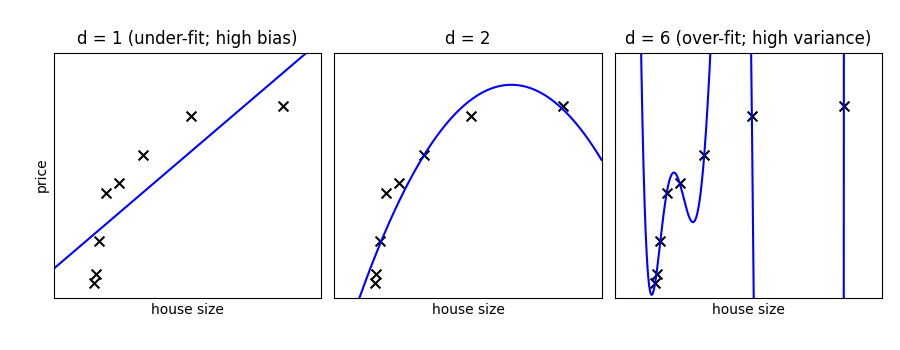
Fit polynomes of different degrees to a dataset: for too small a degree, the model underfits, while for too large a degree, it overfits.

import numpy as np
import matplotlib.pyplot as plt


def generating_func(x, rng=None, error=0.5):
    rng = np.random.default_rng(rng)
    return rng.normal(10 - 1.0 / (x + 0.1), error)

A polynomial regression

from sklearn.pipeline import make_pipeline
from sklearn.linear_model import LinearRegression
from sklearn.preprocessing import PolynomialFeatures

A simple figure to illustrate the problem

n_samples = 8

rng = np.random.default_rng(27446968)
x = 10 ** np.linspace(-2, 0, n_samples)
y = generating_func(x, rng=rng)

x_test = np.linspace(-0.2, 1.2, 1000)

titles = ["d = 1 (under-fit; high bias)", "d = 2", "d = 6 (over-fit; high variance)"]
degrees = [1, 2, 6]

fig = plt.figure(figsize=(9, 3.5))
fig.subplots_adjust(left=0.06, right=0.98, bottom=0.15, top=0.85, wspace=0.05)

for i, d in enumerate(degrees):
    ax = fig.add_subplot(131 + i, xticks=[], yticks=[])
    ax.scatter(x, y, marker="x", c="k", s=50)

    model = make_pipeline(PolynomialFeatures(d), LinearRegression())
    model.fit(x[:, np.newaxis], y)
    ax.plot(x_test, model.predict(x_test[:, np.newaxis]), "-b")

    ax.set_xlim(-0.2, 1.2)
    ax.set_ylim(0, 12)
    ax.set_xlabel("house size")
    if i == 0:
        ax.set_ylabel("price")

    ax.set_title(titles[i])

Generate a larger dataset

from sklearn.model_selection import train_test_split

n_samples = 200
test_size = 0.4
error = 1.0

# randomly sample the data
x = rng.random(n_samples)
y = generating_func(x, rng=rng, error=error)

# split into training, validation, and testing sets.
x_train, x_test, y_train, y_test = train_test_split(x, y, test_size=test_size)

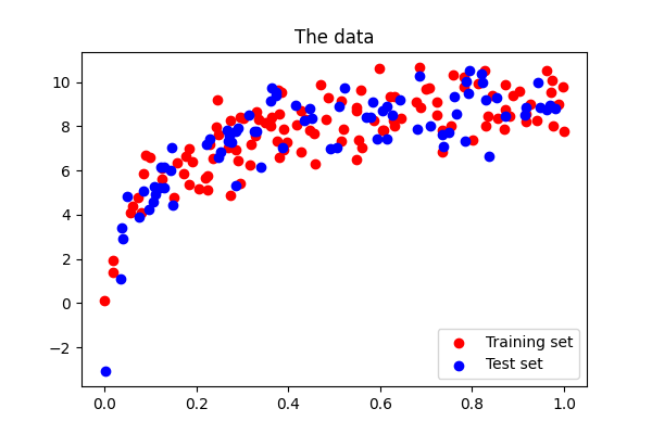
# show the training and validation sets
plt.figure(figsize=(6, 4))
plt.scatter(x_train, y_train, color="red", label="Training set")
plt.scatter(x_test, y_test, color="blue", label="Test set")
plt.title("The data")
plt.legend(loc="best")

<matplotlib.legend.Legend object at 0x7f2925bbe8d0>

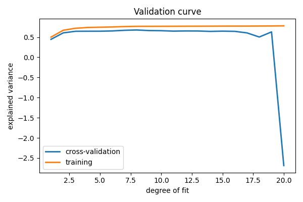
Plot a validation curve

from sklearn.model_selection import validation_curve

degrees = np.arange(1, 21)

model = make_pipeline(PolynomialFeatures(), LinearRegression())

# The parameter to vary is the "degrees" on the pipeline step
# "polynomialfeatures"
train_scores, validation_scores = validation_curve(
    model,
    x[:, np.newaxis],
    y,
    param_name="polynomialfeatures__degree",
    param_range=degrees,
)

# Plot the mean train error and validation error across folds
plt.figure(figsize=(6, 4))
plt.plot(degrees, validation_scores.mean(axis=1), lw=2, label="cross-validation")
plt.plot(degrees, train_scores.mean(axis=1), lw=2, label="training")

plt.legend(loc="best")
plt.xlabel("degree of fit")
plt.ylabel("explained variance")
plt.title("Validation curve")
plt.tight_layout()

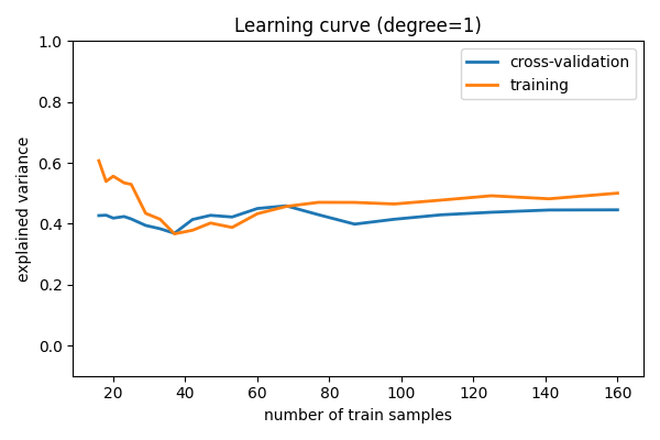
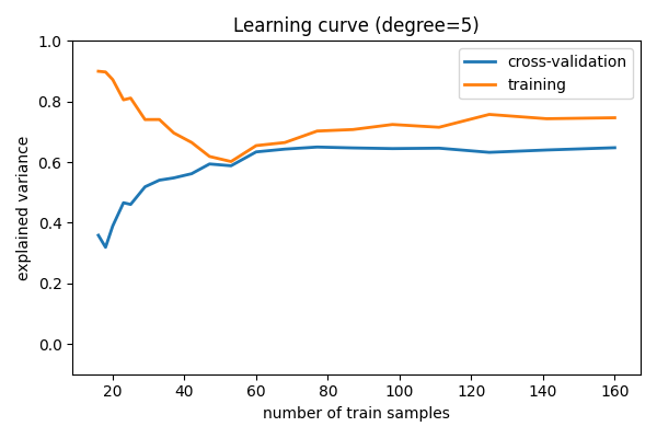
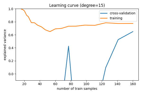
Learning curves

Plot train and test error with an increasing number of samples

# A learning curve for d=1, 5, 15
for d in [1, 5, 15]:
    model = make_pipeline(PolynomialFeatures(degree=d), LinearRegression())

    from sklearn.model_selection import learning_curve

    train_sizes, train_scores, validation_scores = learning_curve(
        model, x[:, np.newaxis], y, train_sizes=np.logspace(-1, 0, 20)
    )

    # Plot the mean train error and validation error across folds
    plt.figure(figsize=(6, 4))
    plt.plot(
        train_sizes, validation_scores.mean(axis=1), lw=2, label="cross-validation"
    )
    plt.plot(train_sizes, train_scores.mean(axis=1), lw=2, label="training")
    plt.ylim(ymin=-0.1, ymax=1)

    plt.legend(loc="best")
    plt.xlabel("number of train samples")
    plt.ylabel("explained variance")
    plt.title("Learning curve (degree=%i)" % d)
    plt.tight_layout()


plt.show()

• 
• 
•