3.4.8.10. Plot fitting a 9th order polynomial

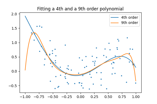
Fits data generated from a 9th order polynomial with model of 4th order and 9th order polynomials, to demonstrate that often simpler models are to be preferred

import numpy as np
import matplotlib.pyplot as plt
from matplotlib.colors import ListedColormap

from sklearn import linear_model

# Create color maps for 3-class classification problem, as with iris
cmap_light = ListedColormap(["#FFAAAA", "#AAFFAA", "#AAAAFF"])
cmap_bold = ListedColormap(["#FF0000", "#00FF00", "#0000FF"])


rng = np.random.default_rng(27446968)
x = 2 * rng.random(100) - 1

f = lambda t: 1.2 * t**2 + 0.1 * t**3 - 0.4 * t**5 - 0.5 * t**9
y = f(x) + 0.4 * rng.normal(size=100)

x_test = np.linspace(-1, 1, 100)

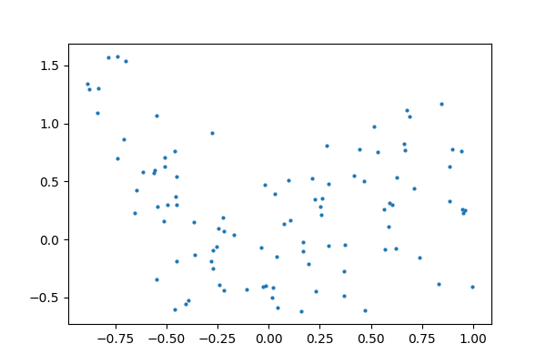
The data

plt.figure(figsize=(6, 4))
plt.scatter(x, y, s=4)

<matplotlib.collections.PathCollection object at 0x7f0921206cd0>

Fitting 4th and 9th order polynomials

For this we need to engineer features: the n_th powers of x:

plt.figure(figsize=(6, 4))
plt.scatter(x, y, s=4)

X = np.array([x**i for i in range(5)]).T
X_test = np.array([x_test**i for i in range(5)]).T
regr = linear_model.LinearRegression()
regr.fit(X, y)
plt.plot(x_test, regr.predict(X_test), label="4th order")

X = np.array([x**i for i in range(10)]).T
X_test = np.array([x_test**i for i in range(10)]).T
regr = linear_model.LinearRegression()
regr.fit(X, y)
plt.plot(x_test, regr.predict(X_test), label="9th order")

plt.legend(loc="best")
plt.axis("tight")
plt.title("Fitting a 4th and a 9th order polynomial")

Text(0.5, 1.0, 'Fitting a 4th and a 9th order polynomial')

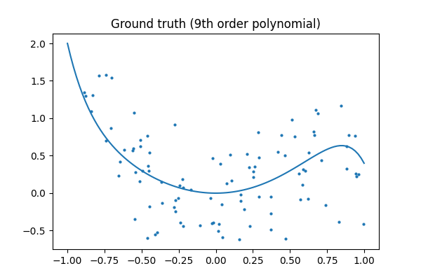
Ground truth

plt.figure(figsize=(6, 4))
plt.scatter(x, y, s=4)
plt.plot(x_test, f(x_test), label="truth")
plt.axis("tight")
plt.title("Ground truth (9th order polynomial)")

plt.show()