3.4.8.7. Plot variance and regularization in linear models

import numpy as np

# Smaller figures
import matplotlib.pyplot as plt

plt.rcParams["figure.figsize"] = (3, 2)

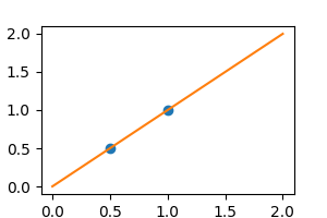
We consider the situation where we have only 2 data point

X = np.c_[0.5, 1].T
y = [0.5, 1]
X_test = np.c_[0, 2].T

Without noise, as linear regression fits the data perfectly

from sklearn import linear_model

regr = linear_model.LinearRegression()
regr.fit(X, y)
plt.plot(X, y, "o")
plt.plot(X_test, regr.predict(X_test))

[<matplotlib.lines.Line2D object at 0x7fb0dd424d10>]

In real life situation, we have noise (e.g. measurement noise) in our data:

rng = np.random.default_rng(27446968)
for _ in range(6):
    noisy_X = X + np.random.normal(loc=0, scale=0.1, size=X.shape)
    plt.plot(noisy_X, y, "o")
    regr.fit(noisy_X, y)
    plt.plot(X_test, regr.predict(X_test))

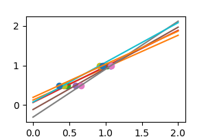
As we can see, our linear model captures and amplifies the noise in the data. It displays a lot of variance.

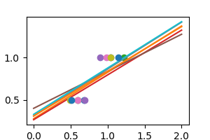
We can use another linear estimator that uses regularization, the Ridge estimator. This estimator regularizes the coefficients by shrinking them to zero, under the assumption that very high correlations are often spurious. The alpha parameter controls the amount of shrinkage used.

regr = linear_model.Ridge(alpha=0.1)
np.random.seed(0)
for _ in range(6):
    noisy_X = X + np.random.normal(loc=0, scale=0.1, size=X.shape)
    plt.plot(noisy_X, y, "o")
    regr.fit(noisy_X, y)
    plt.plot(X_test, regr.predict(X_test))

plt.show()