Simple image blur by convolution with a Gaussian kernel

Blur an an image (../../../../data/elephant.png) using a Gaussian kernel.

Convolution is easy to perform with FFT: convolving two signals boils down to multiplying their FFTs (and performing an inverse FFT).

import numpy as np
import scipy as sp
import matplotlib.pyplot as plt

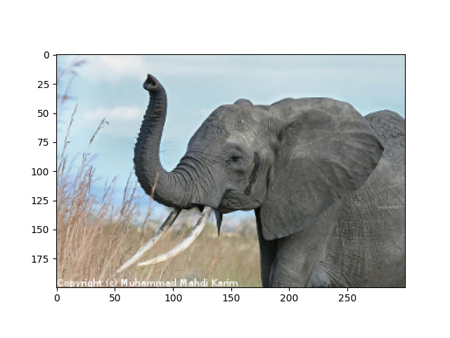
The original image

# read image
img = plt.imread("../../../../data/elephant.png")
plt.figure()
plt.imshow(img)

<matplotlib.image.AxesImage object at 0x7fe9dac4b4d0>

Prepare an Gaussian convolution kernel

# First a 1-D  Gaussian
t = np.linspace(-10, 10, 30)
bump = np.exp(-0.1 * t**2)
bump /= np.trapezoid(bump)  # normalize the integral to 1

# make a 2-D kernel out of it
kernel = bump[:, np.newaxis] * bump[np.newaxis, :]

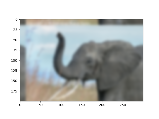
Implement convolution via FFT

# Padded fourier transform, with the same shape as the image
# We use :func:`scipy.fft.fft2` to have a 2D FFT
kernel_ft = sp.fft.fft2(kernel, s=img.shape[:2], axes=(0, 1))

# convolve
img_ft = sp.fft.fft2(img, axes=(0, 1))
# the 'newaxis' is to match to color direction
img2_ft = kernel_ft[:, :, np.newaxis] * img_ft
img2 = sp.fft.ifft2(img2_ft, axes=(0, 1)).real

# clip values to range
img2 = np.clip(img2, 0, 1)

# plot output
plt.figure()
plt.imshow(img2)

<matplotlib.image.AxesImage object at 0x7fe9daf61be0>

Further exercise (only if you are familiar with this stuff):

A “wrapped border” appears in the upper left and top edges of the image. This is because the padding is not done correctly, and does not take the kernel size into account (so the convolution “flows out of bounds of the image”). Try to remove this artifact.

A function to do it: scipy.signal.fftconvolve()

The above exercise was only for didactic reasons: there exists a function in scipy that will do this for us, and probably do a better job: scipy.signal.fftconvolve()

# mode='same' is there to enforce the same output shape as input arrays
# (ie avoid border effects)
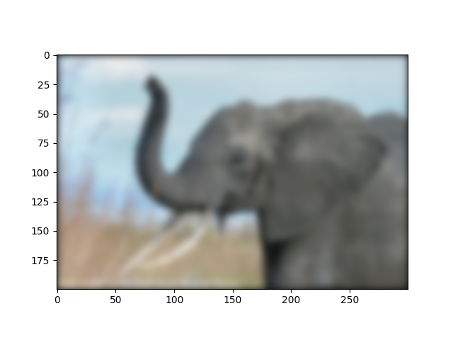
img3 = sp.signal.fftconvolve(img, kernel[:, :, np.newaxis], mode="same")
plt.figure()
plt.imshow(img3)

<matplotlib.image.AxesImage object at 0x7fe9da974170>

Note that we still have a decay to zero at the border of the image. Using scipy.ndimage.gaussian_filter() would get rid of this artifact

plt.show()