The lidar system, data and fit (1 of 2 datasets)

Generate a chart of the data fitted by Gaussian curve

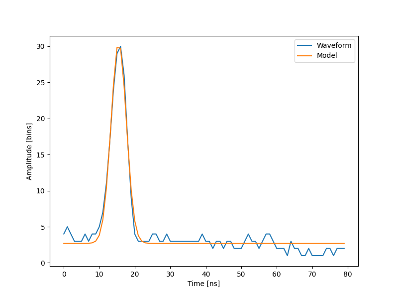
[ 2.70363341 27.82020742 15.47924562  3.05636228]

import numpy as np
import matplotlib.pyplot as plt
import scipy as sp


def model(t, coeffs):
    return coeffs[0] + coeffs[1] * np.exp(-(((t - coeffs[2]) / coeffs[3]) ** 2))


def residuals(coeffs, y, t):
    return y - model(t, coeffs)


waveform_1 = np.load("waveform_1.npy")
t = np.arange(len(waveform_1))

x0 = np.array([3, 30, 15, 1], dtype=float)
x, flag = sp.optimize.leastsq(residuals, x0, args=(waveform_1, t))

print(x)

fig, ax = plt.subplots(figsize=(8, 6))
plt.plot(t, waveform_1, t, model(t, x))
plt.xlabel("Time [ns]")
plt.ylabel("Amplitude [bins]")
plt.legend(["Waveform", "Model"])
plt.show()