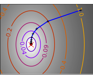
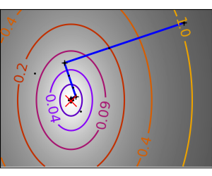
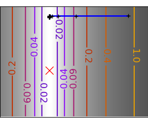
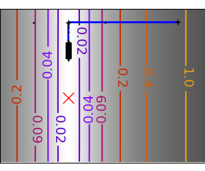
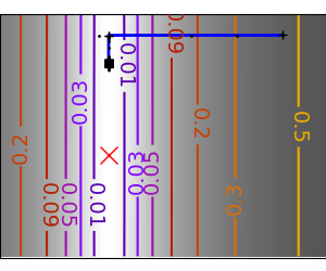
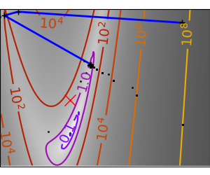
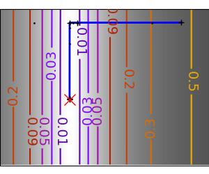
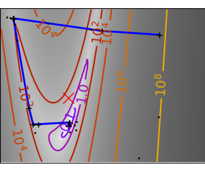
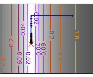
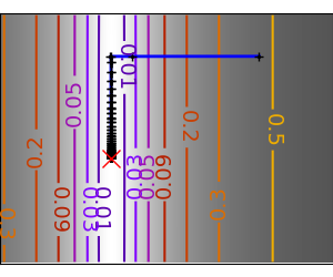
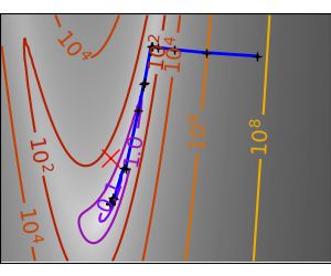
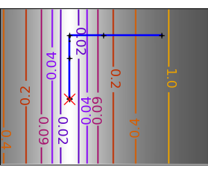
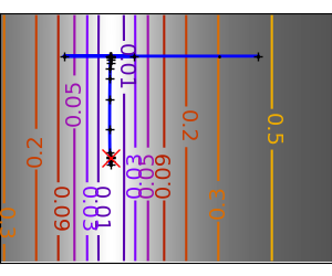
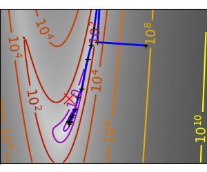
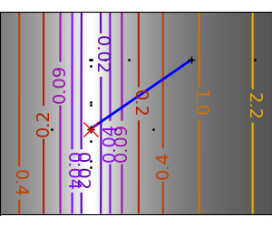
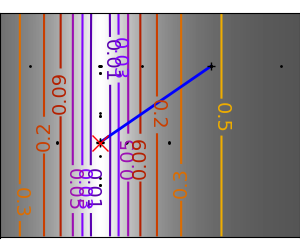
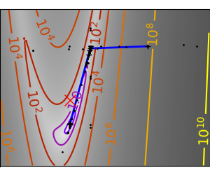
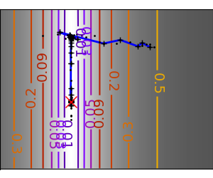
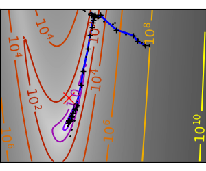
2.7.4.11. Gradient descent

An example demoing gradient descent by creating figures that trace the evolution of the optimizer.

import numpy as np
import matplotlib.pyplot as plt
import scipy as sp

import sys
import os

sys.path.append(os.path.abspath("helper"))
from cost_functions import (
    mk_quad,
    mk_gauss,
    rosenbrock,
    rosenbrock_prime,
    rosenbrock_hessian,
    LoggingFunction,
    CountingFunction,
)

x_min, x_max = -1, 2
y_min, y_max = 2.25 / 3 * x_min - 0.2, 2.25 / 3 * x_max - 0.2

A formatter to print values on contours

def super_fmt(value):
    if value > 1:
        if np.abs(int(value) - value) < 0.1:
            out = f"$10^{{{int(value):d}}}$"
        else:
            out = f"$10^{{{value:.1f}}}$"
    else:
        value = np.exp(value - 0.01)
        if value > 0.1:
            out = f"{value:1.1f}"
        elif value > 0.01:
            out = f"{value:.2f}"
        else:
            out = f"{value:.2e}"
    return out

A gradient descent algorithm do not use: its a toy, use scipy’s optimize.fmin_cg

def gradient_descent(x0, f, f_prime, hessian=None, adaptative=False):
    x_i, y_i = x0
    all_x_i = []
    all_y_i = []
    all_f_i = []

    for i in range(1, 100):
        all_x_i.append(x_i)
        all_y_i.append(y_i)
        all_f_i.append(f([x_i, y_i]))
        dx_i, dy_i = f_prime(np.asarray([x_i, y_i]))
        if adaptative:
            # Compute a step size using a line_search to satisfy the Wolf
            # conditions
            step = sp.optimize.line_search(
                f,
                f_prime,
                np.r_[x_i, y_i],
                -np.r_[dx_i, dy_i],
                np.r_[dx_i, dy_i],
                c2=0.05,
            )
            step = step[0]
            if step is None:
                step = 0
        else:
            step = 1
        x_i += -step * dx_i
        y_i += -step * dy_i
        if np.abs(all_f_i[-1]) < 1e-16:
            break
    return all_x_i, all_y_i, all_f_i


def gradient_descent_adaptative(x0, f, f_prime, hessian=None):
    return gradient_descent(x0, f, f_prime, adaptative=True)


def conjugate_gradient(x0, f, f_prime, hessian=None):
    all_x_i = [x0[0]]
    all_y_i = [x0[1]]
    all_f_i = [f(x0)]

    def store(X):
        x, y = X
        all_x_i.append(x)
        all_y_i.append(y)
        all_f_i.append(f(X))

    sp.optimize.minimize(
        f, x0, jac=f_prime, method="CG", callback=store, options={"gtol": 1e-12}
    )
    return all_x_i, all_y_i, all_f_i


def newton_cg(x0, f, f_prime, hessian):
    all_x_i = [x0[0]]
    all_y_i = [x0[1]]
    all_f_i = [f(x0)]

    def store(X):
        x, y = X
        all_x_i.append(x)
        all_y_i.append(y)
        all_f_i.append(f(X))

    sp.optimize.minimize(
        f,
        x0,
        method="Newton-CG",
        jac=f_prime,
        hess=hessian,
        callback=store,
        options={"xtol": 1e-12},
    )
    return all_x_i, all_y_i, all_f_i


def bfgs(x0, f, f_prime, hessian=None):
    all_x_i = [x0[0]]
    all_y_i = [x0[1]]
    all_f_i = [f(x0)]

    def store(X):
        x, y = X
        all_x_i.append(x)
        all_y_i.append(y)
        all_f_i.append(f(X))

    sp.optimize.minimize(
        f, x0, method="BFGS", jac=f_prime, callback=store, options={"gtol": 1e-12}
    )
    return all_x_i, all_y_i, all_f_i


def powell(x0, f, f_prime, hessian=None):
    all_x_i = [x0[0]]
    all_y_i = [x0[1]]
    all_f_i = [f(x0)]

    def store(X):
        x, y = X
        all_x_i.append(x)
        all_y_i.append(y)
        all_f_i.append(f(X))

    sp.optimize.minimize(
        f, x0, method="Powell", callback=store, options={"ftol": 1e-12}
    )
    return all_x_i, all_y_i, all_f_i


def nelder_mead(x0, f, f_prime, hessian=None):
    all_x_i = [x0[0]]
    all_y_i = [x0[1]]
    all_f_i = [f(x0)]

    def store(X):
        x, y = X
        all_x_i.append(x)
        all_y_i.append(y)
        all_f_i.append(f(X))

    sp.optimize.minimize(
        f, x0, method="Nelder-Mead", callback=store, options={"ftol": 1e-12}
    )
    return all_x_i, all_y_i, all_f_i

Run different optimizers on these problems

levels = {}

for index, ((f, f_prime, hessian), optimizer) in enumerate(
    (
        (mk_quad(0.7), gradient_descent),
        (mk_quad(0.7), gradient_descent_adaptative),
        (mk_quad(0.02), gradient_descent),
        (mk_quad(0.02), gradient_descent_adaptative),
        (mk_gauss(0.02), gradient_descent_adaptative),
        (
            (rosenbrock, rosenbrock_prime, rosenbrock_hessian),
            gradient_descent_adaptative,
        ),
        (mk_gauss(0.02), conjugate_gradient),
        ((rosenbrock, rosenbrock_prime, rosenbrock_hessian), conjugate_gradient),
        (mk_quad(0.02), newton_cg),
        (mk_gauss(0.02), newton_cg),
        ((rosenbrock, rosenbrock_prime, rosenbrock_hessian), newton_cg),
        (mk_quad(0.02), bfgs),
        (mk_gauss(0.02), bfgs),
        ((rosenbrock, rosenbrock_prime, rosenbrock_hessian), bfgs),
        (mk_quad(0.02), powell),
        (mk_gauss(0.02), powell),
        ((rosenbrock, rosenbrock_prime, rosenbrock_hessian), powell),
        (mk_gauss(0.02), nelder_mead),
        ((rosenbrock, rosenbrock_prime, rosenbrock_hessian), nelder_mead),
    )
):
    # Compute a gradient-descent
    x_i, y_i = 1.6, 1.1
    counting_f_prime = CountingFunction(f_prime)
    counting_hessian = CountingFunction(hessian)
    logging_f = LoggingFunction(f, counter=counting_f_prime.counter)
    all_x_i, all_y_i, all_f_i = optimizer(
        np.array([x_i, y_i]), logging_f, counting_f_prime, hessian=counting_hessian
    )

    # Plot the contour plot
    if not max(all_y_i) < y_max:
        x_min *= 1.2
        x_max *= 1.2
        y_min *= 1.2
        y_max *= 1.2
    x, y = np.mgrid[x_min:x_max:100j, y_min:y_max:100j]
    x = x.T
    y = y.T

    plt.figure(index, figsize=(3, 2.5))
    plt.clf()
    plt.axes([0, 0, 1, 1])

    X = np.concatenate((x[np.newaxis, ...], y[np.newaxis, ...]), axis=0)
    z = np.apply_along_axis(f, 0, X)
    log_z = np.log(z + 0.01)
    plt.imshow(
        log_z,
        extent=[x_min, x_max, y_min, y_max],
        cmap=plt.cm.gray_r,
        origin="lower",
        vmax=log_z.min() + 1.5 * log_z.ptp(),
    )
    contours = plt.contour(
        log_z,
        levels=levels.get(f),
        extent=[x_min, x_max, y_min, y_max],
        cmap=plt.cm.gnuplot,
        origin="lower",
    )
    levels[f] = contours.levels
    plt.clabel(contours, inline=1, fmt=super_fmt, fontsize=14)

    plt.plot(all_x_i, all_y_i, "b-", linewidth=2)
    plt.plot(all_x_i, all_y_i, "k+")

    plt.plot(logging_f.all_x_i, logging_f.all_y_i, "k.", markersize=2)

    plt.plot([0], [0], "rx", markersize=12)

    plt.xticks(())
    plt.yticks(())
    plt.xlim(x_min, x_max)
    plt.ylim(y_min, y_max)
    plt.draw()

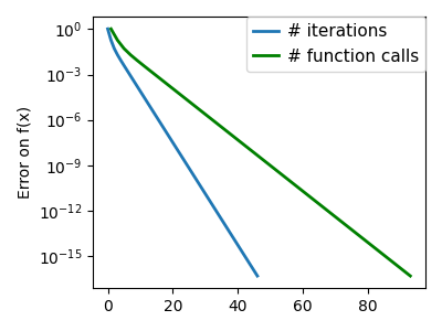
    plt.figure(index + 100, figsize=(4, 3))
    plt.clf()
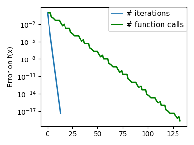
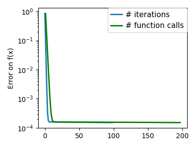
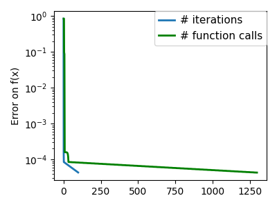
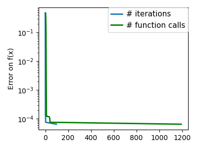
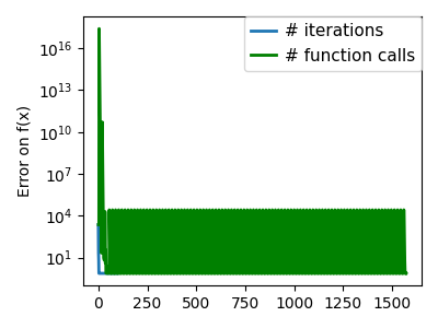
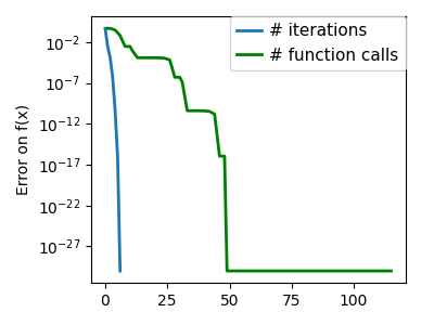
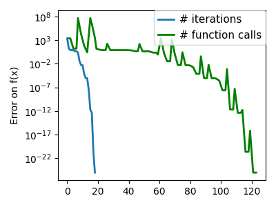
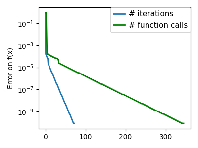
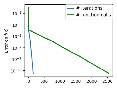
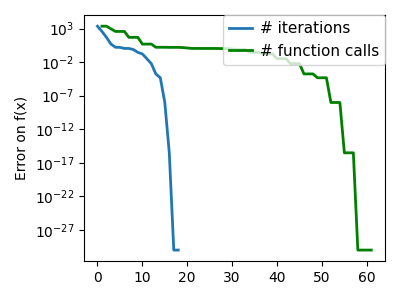
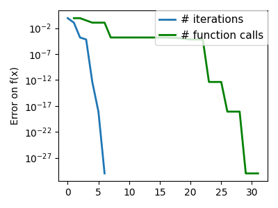
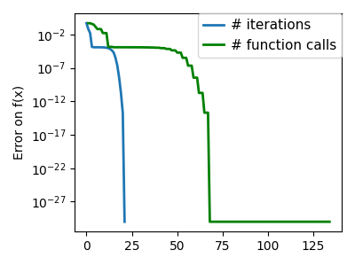
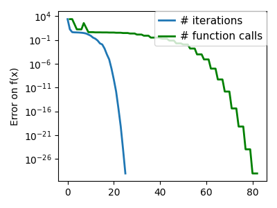
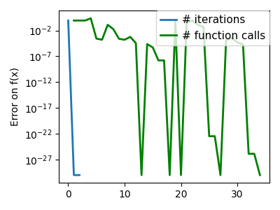
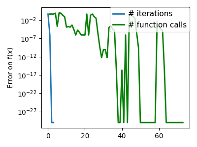
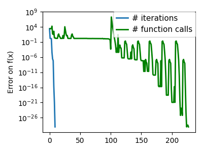
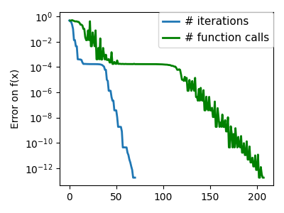
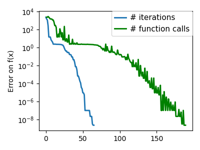
    plt.semilogy(np.maximum(np.abs(all_f_i), 1e-30), linewidth=2, label="# iterations")
    plt.ylabel("Error on f(x)")
    plt.semilogy(
        logging_f.counts,
        np.maximum(np.abs(logging_f.all_f_i), 1e-30),
        linewidth=2,
        color="g",
        label="# function calls",
    )
    plt.legend(
        loc="upper right",
        frameon=True,
        prop={"size": 11},
        borderaxespad=0,
        handlelength=1.5,
        handletextpad=0.5,
    )
    plt.tight_layout()
    plt.draw()

• 
• 
• 
• 
• 
• 
• 
• 
• 
• 
• 
• 
• 
• 
• 
• 
• 
• 
• 
• 
• 
• 
• 
• 
• 
• 
• 
• 
• 
• 
• 
• 
• 
• 
• 
• 
• 
• 

/opt/hostedtoolcache/Python/3.11.9/x64/lib/python3.11/site-packages/scipy/optimize/_linesearch.py:313: LineSearchWarning: The line search algorithm did not converge
  alpha_star, phi_star, old_fval, derphi_star = scalar_search_wolfe2(
/home/runner/work/scientific-python-lectures/scientific-python-lectures/advanced/mathematical_optimization/examples/plot_gradient_descent.py:69: LineSearchWarning: The line search algorithm did not converge
  step = sp.optimize.line_search(
/home/runner/work/scientific-python-lectures/scientific-python-lectures/advanced/mathematical_optimization/examples/plot_gradient_descent.py:233: RuntimeWarning: More than 20 figures have been opened. Figures created through the pyplot interface (`matplotlib.pyplot.figure`) are retained until explicitly closed and may consume too much memory. (To control this warning, see the rcParam `figure.max_open_warning`). Consider using `matplotlib.pyplot.close()`.
  plt.figure(index, figsize=(3, 2.5))
/home/runner/work/scientific-python-lectures/scientific-python-lectures/advanced/mathematical_optimization/examples/plot_gradient_descent.py:178: OptimizeWarning: Unknown solver options: ftol
  sp.optimize.minimize(