1.5.12.15. Optimization of a two-parameter function

import numpy as np


# Define the function that we are interested in
def sixhump(x):
    return (
        (4 - 2.1 * x[0] ** 2 + x[0] ** 4 / 3) * x[0] ** 2
        + x[0] * x[1]
        + (-4 + 4 * x[1] ** 2) * x[1] ** 2
    )


# Make a grid to evaluate the function (for plotting)
xlim = [-2, 2]
ylim = [-1, 1]
x = np.linspace(*xlim)
y = np.linspace(*ylim)
xg, yg = np.meshgrid(x, y)

A 2D image plot of the function

Simple visualization in 2D

import matplotlib.pyplot as plt

plt.figure()
plt.imshow(sixhump([xg, yg]), extent=xlim + ylim, origin="lower")
plt.colorbar()

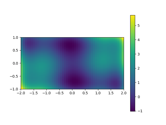
<matplotlib.colorbar.Colorbar object at 0x7f09356f0b10>

A 3D surface plot of the function

from mpl_toolkits.mplot3d import Axes3D

fig = plt.figure()
ax = fig.add_subplot(111, projection="3d")
surf = ax.plot_surface(
    xg,
    yg,
    sixhump([xg, yg]),
    rstride=1,
    cstride=1,
    cmap=plt.cm.viridis,
    linewidth=0,
    antialiased=False,
)

ax.set_xlabel("x")
ax.set_ylabel("y")
ax.set_zlabel("f(x, y)")
ax.set_title("Six-hump Camelback function")

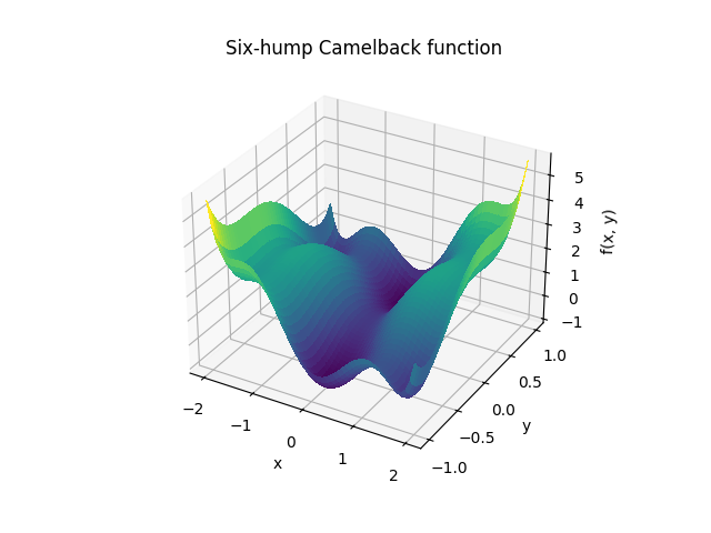
Text(0.5, 1.0, 'Six-hump Camelback function')

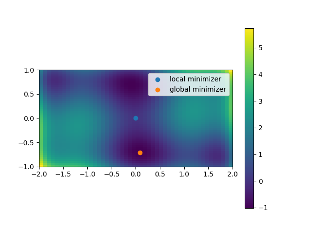
Find minima

import scipy as sp

# local minimization
res_local = sp.optimize.minimize(sixhump, x0=[0, 0])

# global minimization
res_global = sp.optimize.differential_evolution(sixhump, bounds=[xlim, ylim])

plt.figure()
# Show the function in 2D
plt.imshow(sixhump([xg, yg]), extent=xlim + ylim, origin="lower")
plt.colorbar()
# Mark the minima
plt.scatter(res_local.x[0], res_local.x[1], label="local minimizer")
plt.scatter(res_global.x[0], res_global.x[1], label="global minimizer")
plt.legend()
plt.show()