1.5.12.17. A demo of 1D interpolation

• 
• 
• 

# Generate data
import numpy as np

rng = np.random.default_rng(27446968)
measured_time = np.linspace(0, 2 * np.pi, 20)
function = np.sin(measured_time)
noise = rng.normal(loc=0, scale=0.1, size=20)
measurements = function + noise

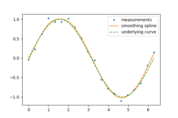
# Smooth the curve and interpolate at new times
import scipy as sp

smoothing_spline = sp.interpolate.make_smoothing_spline(measured_time, measurements)
interpolation_time = np.linspace(0, 2 * np.pi, 200)
smooth_results = smoothing_spline(interpolation_time)

# Plot the data, the interpolant, and the original function
import matplotlib.pyplot as plt

plt.figure(figsize=(6, 4))
plt.plot(measured_time, measurements, ".", ms=6, label="measurements")
plt.plot(interpolation_time, smooth_results, label="smoothing spline")
plt.plot(interpolation_time, np.sin(interpolation_time), "--", label="underlying curve")
plt.legend()
plt.show()

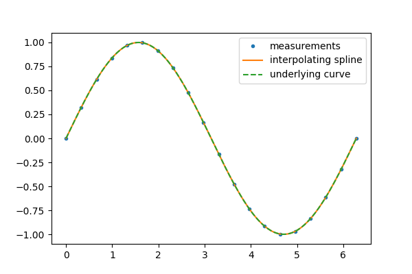
# Fit the data exactly
interp_spline = sp.interpolate.make_interp_spline(measured_time, function)
interp_results = interp_spline(interpolation_time)

# Plot the data, the interpolant, and the original function
plt.figure(figsize=(6, 4))
plt.plot(measured_time, function, ".", ms=6, label="measurements")
plt.plot(interpolation_time, interp_results, label="interpolating spline")
plt.plot(interpolation_time, np.sin(interpolation_time), "--", label="underlying curve")
plt.legend()
plt.show()

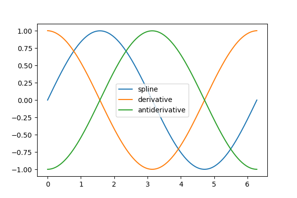
# Plot interpolant, its derivative, and its antiderivative
plt.figure(figsize=(6, 4))
t = interpolation_time
plt.plot(t, interp_spline(t), label="spline")
plt.plot(t, interp_spline.derivative()(t), label="derivative")
plt.plot(t, interp_spline.antiderivative()(t) - 1, label="antiderivative")

plt.legend()
plt.show()