3.4.8.13. Simple visualization and classification of the digits dataset

Plot the first few samples of the digits dataset and a 2D representation built using PCA, then do a simple classification

from sklearn.datasets import load_digits

digits = load_digits()

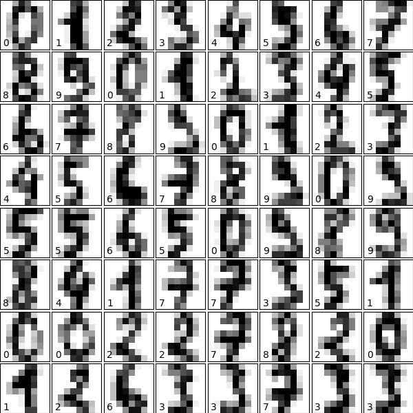
Plot the data: images of digits

Each data in a 8x8 image

import matplotlib.pyplot as plt

fig = plt.figure(figsize=(6, 6))  # figure size in inches
fig.subplots_adjust(left=0, right=1, bottom=0, top=1, hspace=0.05, wspace=0.05)

for i in range(64):
    ax = fig.add_subplot(8, 8, i + 1, xticks=[], yticks=[])
    ax.imshow(digits.images[i], cmap=plt.cm.binary, interpolation="nearest")
    # label the image with the target value
    ax.text(0, 7, str(digits.target[i]))

Plot a projection on the 2 first principal axis

plt.figure()

from sklearn.decomposition import PCA

pca = PCA(n_components=2)
proj = pca.fit_transform(digits.data)
plt.scatter(proj[:, 0], proj[:, 1], c=digits.target, cmap="Paired")
plt.colorbar()

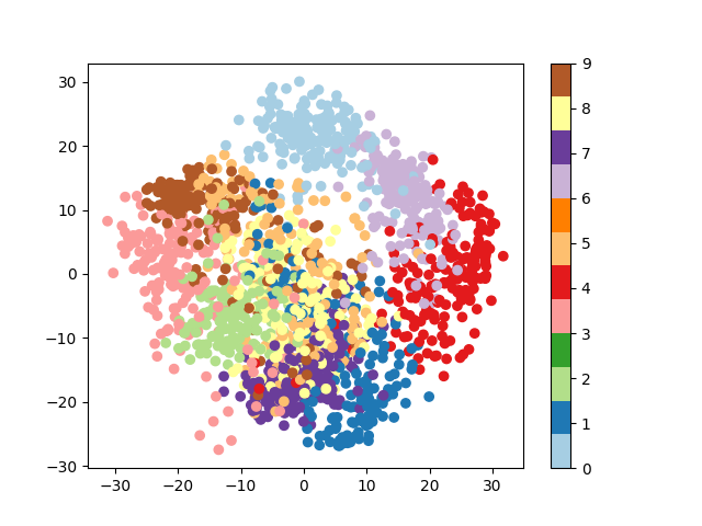
<matplotlib.colorbar.Colorbar object at 0x7fb74d07a990>

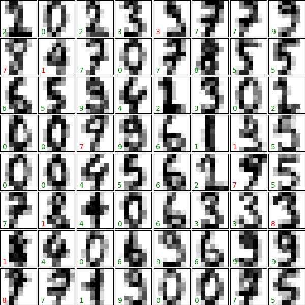
Classify with Gaussian naive Bayes

from sklearn.naive_bayes import GaussianNB
from sklearn.model_selection import train_test_split

# split the data into training and validation sets
X_train, X_test, y_train, y_test = train_test_split(digits.data, digits.target)

# train the model
clf = GaussianNB()
clf.fit(X_train, y_train)

# use the model to predict the labels of the test data
predicted = clf.predict(X_test)
expected = y_test

# Plot the prediction
fig = plt.figure(figsize=(6, 6))  # figure size in inches
fig.subplots_adjust(left=0, right=1, bottom=0, top=1, hspace=0.05, wspace=0.05)

# plot the digits: each image is 8x8 pixels
for i in range(64):
    ax = fig.add_subplot(8, 8, i + 1, xticks=[], yticks=[])
    ax.imshow(X_test.reshape(-1, 8, 8)[i], cmap=plt.cm.binary, interpolation="nearest")

    # label the image with the target value
    if predicted[i] == expected[i]:
        ax.text(0, 7, str(predicted[i]), color="green")
    else:
        ax.text(0, 7, str(predicted[i]), color="red")

Quantify the performance

First print the number of correct matches

matches = predicted == expected
print(matches.sum())

395

The total number of data points

print(len(matches))

450

And now, the ration of correct predictions

matches.sum() / float(len(matches))

np.float64(0.8777777777777778)

Print the classification report

from sklearn import metrics

print(metrics.classification_report(expected, predicted))

              precision    recall  f1-score   support

           0       0.97      0.95      0.96        37
           1       0.83      0.85      0.84        41
           2       0.89      0.84      0.86        49
           3       0.93      0.83      0.88        47
           4       0.93      0.90      0.92        42
           5       0.89      0.95      0.92        42
           6       0.98      0.97      0.97        60
           7       0.81      0.98      0.88        47
           8       0.65      0.87      0.75        39
           9       0.97      0.63      0.76        46

    accuracy                           0.88       450
   macro avg       0.89      0.88      0.87       450
weighted avg       0.89      0.88      0.88       450

Print the confusion matrix

print(metrics.confusion_matrix(expected, predicted))

plt.show()

[[35  0  0  0  1  0  0  1  0  0]
 [ 0 35  0  0  0  0  1  1  4  0]
 [ 0  1 41  0  0  0  0  0  7  0]
 [ 0  0  2 39  0  1  0  2  2  1]
 [ 0  1  0  0 38  0  0  2  1  0]
 [ 0  0  0  0  1 40  0  1  0  0]
 [ 0  0  1  0  1  0 58  0  0  0]
 [ 0  0  0  0  0  1  0 46  0  0]
 [ 0  2  0  1  0  1  0  1 34  0]
 [ 1  3  2  2  0  2  0  3  4 29]]