2.7.4.8. Constraint optimization: visualizing the geometry

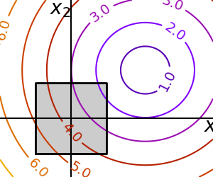
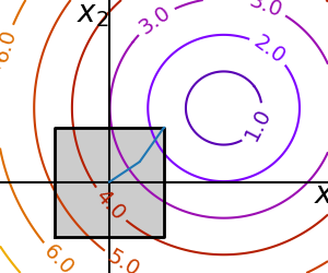
A small figure explaining optimization with constraints

• 
• 

import numpy as np
import matplotlib.pyplot as plt
import scipy as sp

x, y = np.mgrid[-2.9:5.8:0.05, -2.5:5:0.05]
x = x.T
y = y.T

for i in (1, 2):
    # Create 2 figure: only the second one will have the optimization
    # path
    plt.figure(i, figsize=(3, 2.5))
    plt.clf()
    plt.axes([0, 0, 1, 1])

    contours = plt.contour(
        np.sqrt((x - 3) ** 2 + (y - 2) ** 2),
        extent=[-3, 6, -2.5, 5],
        cmap=plt.cm.gnuplot,
    )
    plt.clabel(contours, inline=1, fmt="%1.1f", fontsize=14)
    plt.plot(
        [-1.5, -1.5, 1.5, 1.5, -1.5], [-1.5, 1.5, 1.5, -1.5, -1.5], "k", linewidth=2
    )
    plt.fill_between([-1.5, 1.5], [-1.5, -1.5], [1.5, 1.5], color=".8")
    plt.axvline(0, color="k")
    plt.axhline(0, color="k")

    plt.text(-0.9, 4.4, "$x_2$", size=20)
    plt.text(5.6, -0.6, "$x_1$", size=20)
    plt.axis("equal")
    plt.axis("off")

# And now plot the optimization path
accumulator = []


def f(x):
    # Store the list of function calls
    accumulator.append(x)
    return np.sqrt((x[0] - 3) ** 2 + (x[1] - 2) ** 2)


# We don't use the gradient, as with the gradient, L-BFGS is too fast,
# and finds the optimum without showing us a pretty path
def f_prime(x):
    r = np.sqrt((x[0] - 3) ** 2 + (x[0] - 2) ** 2)
    return np.array(((x[0] - 3) / r, (x[0] - 2) / r))


sp.optimize.minimize(
    f, np.array([0, 0]), method="L-BFGS-B", bounds=((-1.5, 1.5), (-1.5, 1.5))
)

accumulated = np.array(accumulator)
plt.plot(accumulated[:, 0], accumulated[:, 1])

plt.show()