2.7.4.6. Optimization with constraints

An example showing how to do optimization with general constraints using SLSQP and cobyla.

import numpy as np
import matplotlib.pyplot as plt
import scipy as sp

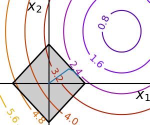
x, y = np.mgrid[-2.03:4.2:0.04, -1.6:3.2:0.04]
x = x.T
y = y.T

plt.figure(1, figsize=(3, 2.5))
plt.clf()
plt.axes([0, 0, 1, 1])

contours = plt.contour(
    np.sqrt((x - 3) ** 2 + (y - 2) ** 2),
    extent=[-2.03, 4.2, -1.6, 3.2],
    cmap=plt.cm.gnuplot,
)
plt.clabel(contours, inline=1, fmt="%1.1f", fontsize=14)
plt.plot([-1.5, 0, 1.5, 0, -1.5], [0, 1.5, 0, -1.5, 0], "k", linewidth=2)
plt.fill_between([-1.5, 0, 1.5], [0, -1.5, 0], [0, 1.5, 0], color=".8")
plt.axvline(0, color="k")
plt.axhline(0, color="k")

plt.text(-0.9, 2.8, "$x_2$", size=20)
plt.text(3.6, -0.6, "$x_1$", size=20)
plt.axis("tight")
plt.axis("off")

# And now plot the optimization path
accumulator = []


def f(x):
    # Store the list of function calls
    accumulator.append(x)
    return np.sqrt((x[0] - 3) ** 2 + (x[1] - 2) ** 2)


def constraint(x):
    return np.atleast_1d(1.5 - np.sum(np.abs(x)))


sp.optimize.minimize(
    f, np.array([0, 0]), method="SLSQP", constraints={"fun": constraint, "type": "ineq"}
)

accumulated = np.array(accumulator)
plt.plot(accumulated[:, 0], accumulated[:, 1])

plt.show()