3.1.6.4. Simple Regression

Fit a simple linear regression using ‘statsmodels’, compute corresponding p-values.

# Original author: Thomas Haslwanter

import numpy as np
import matplotlib.pyplot as plt
import pandas

# For statistics. Requires statsmodels 5.0 or more
from statsmodels.formula.api import ols

# Analysis of Variance (ANOVA) on linear models
from statsmodels.stats.anova import anova_lm

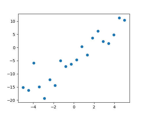
Generate and show the data

x = np.linspace(-5, 5, 20)

# To get reproducible values, provide a seed value
rng = np.random.default_rng(27446968)

y = -5 + 3 * x + 4 * np.random.normal(size=x.shape)

# Plot the data
plt.figure(figsize=(5, 4))
plt.plot(x, y, "o")

[<matplotlib.lines.Line2D object at 0x7f0613ce4440>]

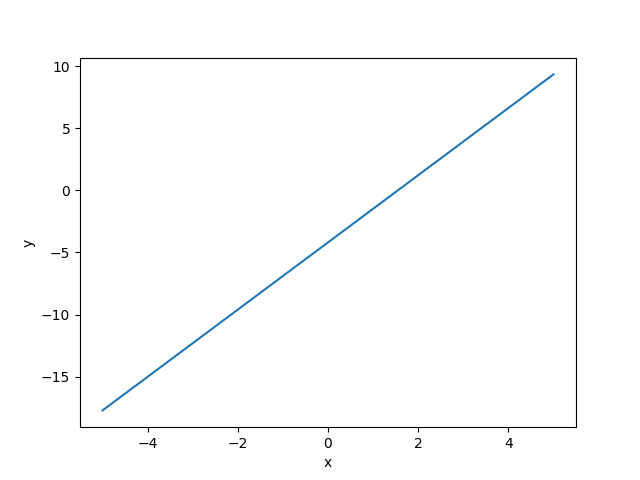
Multilinear regression model, calculating fit, P-values, confidence intervals etc.

# Convert the data into a Pandas DataFrame to use the formulas framework
# in statsmodels
data = pandas.DataFrame({"x": x, "y": y})

# Fit the model
model = ols("y ~ x", data).fit()

# Print the summary
print(model.summary())

# Perform analysis of variance on fitted linear model
anova_results = anova_lm(model)

print("\nANOVA results")
print(anova_results)

                            OLS Regression Results
==============================================================================
Dep. Variable:                      y   R-squared:                       0.845
Model:                            OLS   Adj. R-squared:                  0.836
Method:                 Least Squares   F-statistic:                     97.76
Date:                Tue, 29 Apr 2025   Prob (F-statistic):           1.06e-08
Time:                        04:12:06   Log-Likelihood:                -53.560
No. Observations:                  20   AIC:                             111.1
Df Residuals:                      18   BIC:                             113.1
Df Model:                           1
Covariance Type:            nonrobust
==============================================================================
                 coef    std err          t      P>|t|      [0.025      0.975]
------------------------------------------------------------------------------
Intercept     -4.1877      0.830     -5.044      0.000      -5.932      -2.444
x              2.7046      0.274      9.887      0.000       2.130       3.279
==============================================================================
Omnibus:                        1.871   Durbin-Watson:                   1.930
Prob(Omnibus):                  0.392   Jarque-Bera (JB):                0.597
Skew:                           0.337   Prob(JB):                        0.742
Kurtosis:                       3.512   Cond. No.                         3.03
==============================================================================

Notes:
[1] Standard Errors assume that the covariance matrix of the errors is correctly specified.

ANOVA results
            df       sum_sq      mean_sq          F        PR(>F)
x          1.0  1347.476043  1347.476043  97.760281  1.062847e-08
Residual  18.0   248.102486    13.783471        NaN           NaN

Plot the fitted model

# Retrieve the parameter estimates
offset, coef = model._results.params
plt.plot(x, x * coef + offset)
plt.xlabel("x")
plt.ylabel("y")

plt.show()