3.1.6.5. Multiple Regression

Calculate using ‘statsmodels’ just the best fit, or all the corresponding statistical parameters.

Also shows how to make 3d plots.

# Original author: Thomas Haslwanter

import numpy as np
import matplotlib.pyplot as plt
import pandas

# For 3d plots. This import is necessary to have 3D plotting below
from mpl_toolkits.mplot3d import Axes3D

# For statistics. Requires statsmodels 5.0 or more
from statsmodels.formula.api import ols

# Analysis of Variance (ANOVA) on linear models
from statsmodels.stats.anova import anova_lm

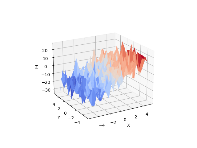
Generate and show the data

x = np.linspace(-5, 5, 21)
# We generate a 2D grid
X, Y = np.meshgrid(x, x)

# To get reproducible values, provide a seed value
rng = np.random.default_rng(27446968)

# Z is the elevation of this 2D grid
Z = -5 + 3 * X - 0.5 * Y + 8 * np.random.normal(size=X.shape)

# Plot the data
ax: Axes3D = plt.figure().add_subplot(projection="3d")
surf = ax.plot_surface(X, Y, Z, cmap="coolwarm", rstride=1, cstride=1)
ax.view_init(20, -120)
ax.set_xlabel("X")
ax.set_ylabel("Y")
ax.set_zlabel("Z")

Text(-0.10764513121260137, 0.009865032686848034, 'Z')

Multilinear regression model, calculating fit, P-values, confidence intervals etc.

# Convert the data into a Pandas DataFrame to use the formulas framework
# in statsmodels

# First we need to flatten the data: it's 2D layout is not relevant.
X = X.flatten()
Y = Y.flatten()
Z = Z.flatten()

data = pandas.DataFrame({"x": X, "y": Y, "z": Z})

# Fit the model
model = ols("z ~ x + y", data).fit()

# Print the summary
print(model.summary())

print("\nRetrieving manually the parameter estimates:")
print(model._results.params)
# should be array([-4.99754526,  3.00250049, -0.50514907])

# Perform analysis of variance on fitted linear model
anova_results = anova_lm(model)

print("\nANOVA results")
print(anova_results)

plt.show()

                            OLS Regression Results
==============================================================================
Dep. Variable:                      z   R-squared:                       0.579
Model:                            OLS   Adj. R-squared:                  0.577
Method:                 Least Squares   F-statistic:                     300.7
Date:                Tue, 06 May 2025   Prob (F-statistic):           6.43e-83
Time:                        06:48:51   Log-Likelihood:                -1552.0
No. Observations:                 441   AIC:                             3110.
Df Residuals:                     438   BIC:                             3122.
Df Model:                           2
Covariance Type:            nonrobust
==============================================================================
                 coef    std err          t      P>|t|      [0.025      0.975]
------------------------------------------------------------------------------
Intercept     -4.4332      0.390    -11.358      0.000      -5.200      -3.666
x              3.0861      0.129     23.940      0.000       2.833       3.340
y             -0.6856      0.129     -5.318      0.000      -0.939      -0.432
==============================================================================
Omnibus:                        0.560   Durbin-Watson:                   1.967
Prob(Omnibus):                  0.756   Jarque-Bera (JB):                0.651
Skew:                          -0.077   Prob(JB):                        0.722
Kurtosis:                       2.893   Cond. No.                         3.03
==============================================================================

Notes:
[1] Standard Errors assume that the covariance matrix of the errors is correctly specified.

Retrieving manually the parameter estimates:
[-4.43322435  3.08614608 -0.68556194]

ANOVA results
             df        sum_sq       mean_sq           F        PR(>F)
x           1.0  38501.973182  38501.973182  573.111646  1.365553e-81
y           1.0   1899.955512   1899.955512   28.281320  1.676135e-07
Residual  438.0  29425.094352     67.180581         NaN           NaN